

人工智能(Pytorch)搭建模型5-注意力机制模型的构建与GRU模型融合应用
大家好,我是微学AI,今天给大家介绍一下人工智能(Pytorch)搭建模型5-注意力机制模型的构建与GRU模型融合应用。注意力机制是一种神经网络模型,在序列到序列的任务中,可以帮助解决输入序列较长时难以获取全局信息的问题。该模型通过对输入序列不同部分赋予不同的权重,以便在每个时间步骤上更好地关注需要处理的信息。在编码器-解码器(Encoder-Decoder)框架中,编码器将输入序列映射为一系列向量,而解码器则在每个时间步骤上生成输出序列。在此过程中,解码器需要对编码器的所有时刻进行“注意”,以了解哪些输入对当前时间步骤最重要。
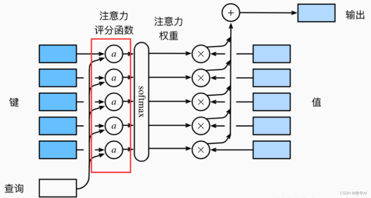
在注意力机制中,解码器会计算每个编码器输出与当前解码器隐藏状态之间的相关度,并将其转化为注意力权重,以确定每个编码器输出对当前时刻解码器状态的贡献。这些权重被用于加权求和编码器输出,从而得到一个上下文向量,该向量包含有关输入序列的重要信息,有助于提高模型的性能和泛化能力。
一、注意力机制模型构建
# 1. 导入所需库
import torch
import torch.nn as nn
import torch.optim as optim
import numpy as np
from torch.utils.data import Dataset, DataLoader
class Attention(nn.Module):
    def __init__(self, hidden_size):
        super(Attention, self).__init__()
        self.hidden_size = hidden_size
        self.attn = nn.Linear(self.hidden_size * 2, hidden_size)
        self.v = nn.Linear(hidden_size, 1, bias=False)
    def forward(self, hidden, encoder_outputs):
        max_len = encoder_outputs.size(1)
        repeated_hidden = hidden.unsqueeze(1).repeat(1, max_len, 1)
        energy = torch.tanh(self.attn(torch.cat((repeated_hidden, encoder_outputs), dim=2)))
        attention_scores = self.v(energy).squeeze(2)
        attention_weights = nn.functional.softmax(attention_scores, dim=1)
        context_vector = (encoder_outputs * attention_weights.unsqueeze(2)).sum(dim=1)
        return context_vector, attention_weights
以上Attention类是注意力机制的神经网络模型,该模型接收两个输入参数:隐藏状态和编码器输出。其中,隐藏状态是解码器中上一个时间步骤的输出,而编码器输出是编码器模型对输入序列进行编码后的输出。编码器输出和隐藏状态被用于计算上下文向量和注意力权重。通过将隐藏状态和编码器输出进行拼接,然后将结果通过线性层进行处理,并使用tanh激活函数后得到能量矩阵(energy)。接着,使用另一个线性层(self.v)将能量矩阵转换成注意力得分(attention scores),并使用softmax函数转换成注意力权重(attention weights)。最后,根据注意力权重对编码器输出进行加权组合得到上下文向量。
整个过程可以简单概括为:先将隐藏状态和编码器输出连接起来,然后使用线性转换和tanh激活函数计算能量矩阵,再使用线性转换和softmax函数计算注意力权重,最后使用注意力权重对编码器输出进行加权组合得到上下文向量。
二、GRU模型构建+注意力机制
class GRUModel(nn.Module):
    def __init__(self, input_size, hidden_size, output_size, num_layers, dropout=0.5):
        super(GRUModel, self).__init__()
        self.hidden_size = hidden_size
        self.num_layers = num_layers
        self.gru = nn.GRU(input_size, hidden_size, num_layers, batch_first=True, dropout=dropout)
        self.attention = Attention(hidden_size)
        self.fc = nn.Linear(hidden_size, output_size)
        self.dropout = nn.Dropout(dropout)
    def forward(self, x):
        h0 = torch.zeros(self.num_layers, x.size(0), self.hidden_size)
        out, hidden = self.gru(x, h0)
        out, attention_weights = self.attention(hidden[-1], out)
        out = self.dropout(out)
        out = self.fc(out)
        return out
GRUModel类的初始化方法中,先调用了父类构造函数初始化。然后定义了一个GRU层,并将其输出传入Attention类中计算上下文向量和注意力权重。最后将上下文向量送入一个线性层,并加上dropout操作,为了防止过拟合现象,然后输出模型的预测结果。通过这个模型的设计,我们可以将输入序列和输出序列的长度变化对模型的性能影响降到最小,并且利用注意力机制使模型能够更好的关注序列中的重要信息。
三、数据生成与加载
# 3. 准备数据集
class SampleDataset(Dataset):
    def __init__(self):
        self.sequences = []
        self.labels = []
        for _ in range(1000):
            seq = torch.randn(10, 5)
            label = torch.zeros(2)
            if seq.sum() > 0:
                label[0] = 1
            else:
                label[1] = 1
            self.sequences.append(seq)
            self.labels.append(label)
    def __len__(self):
        return len(self.sequences)
    def __getitem__(self, idx):
        return self.sequences[idx], self.labels[idx]
train_set_split = int(0.8 * len(SampleDataset()))
train_set, test_set = torch.utils.data.random_split(SampleDataset(),
     [train_set_split, len(SampleDataset()) - train_set_split])
train_loader = DataLoader(train_set, batch_size=32, shuffle=True)
test_loader = DataLoader(test_set, batch_size=32, shuffle=False)
四、模型训练
# 4. 定义训练过程
def train(model, loader, criterion, optimizer, device):
    model.train()
    running_loss = 0.0
    correct = 0
    total = 0
    for batch_idx, (inputs, labels) in enumerate(loader):
        inputs, labels = inputs.to(device), labels.to(device)
        optimizer.zero_grad()
        outputs = model(inputs)
        loss = criterion(outputs, labels)
        loss.backward()
        optimizer.step()
        running_loss += loss.item()
        _, predicted = torch.max(outputs, 1)
        _, true_labels = torch.max(labels, 1)
        total += true_labels.size(0)
        correct += (predicted == true_labels).sum().item()
    print("Train Loss: {:.4f}, Acc: {:.2f}%".format(running_loss / (batch_idx + 1), 100 * correct / total))
# 5. 定义评估过程
def evaluate(model, loader, criterion, device):
    model.eval()
    running_loss = 0.0
    correct = 0
    total = 0
    with torch.no_grad():
        for batch_idx, (inputs, labels) in enumerate(loader):
            inputs, labels = inputs.to(device), labels.to(device)
            outputs = model(inputs)
            loss = criterion(outputs, labels)
            running_loss += loss.item()
            _, predicted = torch.max(outputs, 1)
            _, true_labels = torch.max(labels, 1)
            total += true_labels.size(0)
            correct += (predicted == true_labels).sum().item()
    print("Test Loss: {:.4f}, Acc: {:.2f}%".format(running_loss / (batch_idx + 1), 100 * correct / total))
# 6. 训练模型并评估
device = "cuda" if torch.cuda.is_available() else "cpu"
model = GRUModel(input_size=5, hidden_size=10, output_size=2, num_layers=1).to(device)
criterion = nn.BCEWithLogitsLoss()
optimizer = optim.Adam(model.parameters(), lr=1e-3)
num_epochs = 100
for epoch in range(num_epochs):
    print("Epoch {}/{}".format(epoch + 1, num_epochs))
    train(model, train_loader, criterion, optimizer, device)
    evaluate(model, test_loader, criterion, device)
运行结果:
Epoch 97/100
Train Loss: 0.0264, Acc: 99.75%
Test Loss: 0.1267, Acc: 94.50%
Epoch 98/100
Train Loss: 0.0294, Acc: 99.75%
Test Loss: 0.1314, Acc: 95.00%
Epoch 99/100
Train Loss: 0.0286, Acc: 99.75%
Test Loss: 0.1280, Acc: 94.50%
Epoch 100/100
Train Loss: 0.0286, Acc: 99.75%
Test Loss: 0.1324, Acc: 95.50%
")
")
")
")
还没有评论,来说两句吧...